Perceptual Robotics: Beginner

0.Description of the apparatus

Robotic platform:

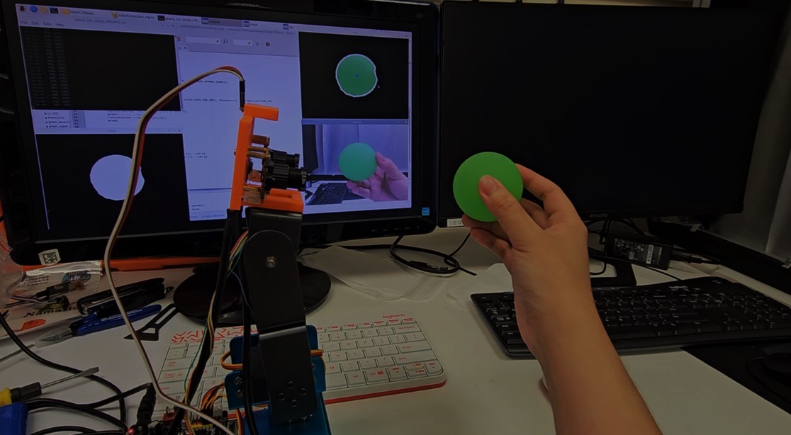
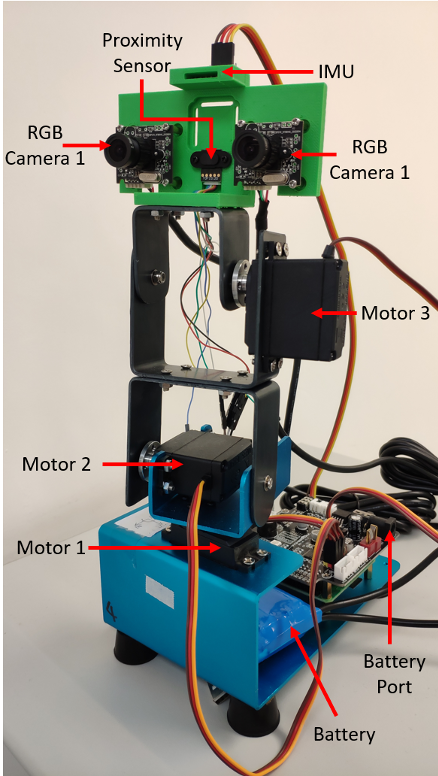
Robotic platform Mingo has 3 degrees of freedoms controlled by 3 step motors. It is equipped with 2 RGB cameras, 1 proximity sensor and 1 IMU. Its controller is Raspberry Pi 4B, a strong single board computer which is capable of motor control, image processing and so on. A Unix-like operating system Raspbian is pre-installed in the Raspberry Pi 4B.

All the example codes are in “Demo” folder on Desktop.

Development Environment:

• How to run code?

  • Open any python codes in Demos folder
  • The system will open Geany (Integrated Development Environment, IDE) shown as below:
  • 
  • you can click the this button in the toolbar or click ->Build -> Execute (F5 is hotkey) in manubar to execute the python code. (The system will run the code with python2 by default. )
  • 

• How to specitify python3 to run code?

  Since some demo codes need advanced libaries that only work with python3, it's necessary to set python3 to execute the corresponding codes. The steps are as follows:

  • click ->Build -> Set Build Commands in manubar and set "ExecutePy3" in Execute commands as below:
  • 
  • Then check the newly added item "ExecutePy3" under Build menu.
  • 

1.Intro to Python

Python is a powerful programming language ideal for scripting and rapid application development. It is used in web development (like: Django and Bottle), scientific and mathematical computing (Orange, SymPy, NumPy) to desktop graphical user Interfaces (Pygame, Panda3D).

This tutorial introduces you to the basic concepts and features of Python 3. After reading the tutorial, you will be able to read and write basic Python programs, and explore Python in depth on your own.

https://www.programiz.com/python-programming/tutorial

2.OpenCV Basics

Following the instruction, you will learn how to open an RGB camera, how to read and save a picture, and how a specific color is selected and extracted.

Open “OpenCVBasic” folder

1. Open cameras

• Connect two cameras to the Raspberry Pi through USB 3.0 ports

• Run “openCamera.py”

• Press “q” to exit

• Change “cap = cv2.VideoCapture(0)” to “cap = cv2.VideoCapture(2)”

• Run “openCamera.py” again

• Press “q” to exit

   

2. Save images

• Run “capture.py”

• Press “c” to capture an image

• Press “q” to exit

• Check the captured image “pic.png” in the same folder

   

3. Read & write images

• Run “ReadAndWrite_img.py”

• Check difference between two images

• Press “q” to exit

• Check “picture.jpg” and“picture1.jpg” in the same folder

   

4. HSV Color Space

In this section, we will develop a basic intuition of HSV color space. HSV (hue, saturation, value) is an alternative representation of the RGB color model, designed in the 1970s by computer graphics researchers to more closely align with the way human vision perceives color-making attributes. In this model, colors of each hue are arranged in a radial slice, around a central axis of neutral colors which ranges from black at the bottom to white at the top. The HSV representation models the way paints of different colors mix together, with the saturation dimension resembling various tints of brightly colored paint, and the value dimension resembling the mixture of those paints with varying amounts of black or white paint.

1. Run “colorSelection_HSV.py”

2. Set “S” and “V” value to “255”

3. Set “H” value from “0” to “255”

4. Try different combinations of “H”, “S”, “Vs” value

5. Press “q” to exit the program.

5. Color Extraction

In this section, we will learn how to extract green color from the video input from the RGB camera

1. Run “colorExtraction.py” in the terminal. Put a green ball in the front of the camera. You should see three windows “original”, “mask” and “res” as shown below.

   

2. Press “s” to save three images of the windows respectively.

3.Camera Calibration

In this section, you will learn the basic knowledge about camera calibration, and calibrate two cameras by yourself.

Open “StereoCallibration” folder

1. Camera distortion

Today’s cheap pinhole cameras introduces a lot of distortion to images. Two major distortions are radial distortion and tangential distortion. Due to radial distortion, straight lines will appear curved. Its effect is more as we move away from the center of image. For example, one image is shown below, where two edges of a chess board are marked with red lines. But you can see that border is not a straight line and doesn’t match with the red line. All the expected straight lines are bulged out.

This distortion is solved as follows:

$\begin{array}{l} x_{\text {corrected }}=x\left(1+k_{1} r^{2}+k_{2} r^{4}+k_{3} r^{6}\right) \\ y_{\text {corrected }}=y\left(1+k_{1} r^{2}+k_{2} r^{4}+k_{3} r^{6}\right) \end{array}$

Similarly, another distortion is the tangential distortion which occurs because image taking lenses are not aligned perfectly parallel to the imaging plane. So some areas in image may look nearer than expected. It is solved as below:

$\begin{array}{l} x_{\text {corrected }}=x+\left[2 p_{1} x y+p_{2}\left(r^{2}+2 x^{2}\right)\right]. \\ y_{\text {corrected }}=y+\left[p_{1}\left(r^{2}+2 y^{2}\right)+2 p_{2} x y\right]. \end{array}$

In short, we need to find five parameters, known as distortion coefficients, given by:

$\text { Distortion coefficients }=\left(k_{1}, k_{2}, p_{1}, p_{2}, k_{3}\right)$

For stereo applications, these distortions need to be corrected first. To find all these parameters, what we have to do is to provide some sample images of a well-defined pattern (e.g., chess board). We find some specific points in it (square corners in chess board). We know its coordinates in real world space and we know its coordinates in image. With these data, some mathematical problem is solved in background to get the distortion coefficients. That is the summary of the whole story. For better results, we need at least 20 test patterns. In addition to this, we need to find a few more information, like intrinsic parameters of a camera.

2. Capture images of calibration board

1. Run “capture_two(ste).py”
2. Place the calibration chess board in the front of two cameras. Make sure two cameras can both see the board completely.
3. Press “c” to capture images.
4. Change the position and orientation of the chess board, repeat step (2)-(4) at least 20 times to capture enough images for calibration
5. Press “q” to exit

3. Calculate and record distortion and camera intrinsic parameters

1. Run “stereo_callibration.py”

2. Record the printed results, including

   • Left camera intrinsic parameters a 3x3 Matrix (Following ‘Intrinsic_mtx_left(K_left)’)
   • Left camera distortion parameters 1x5 Vector (Following 'dist_left’)
   • Right camera intrinsic parameters 3x3 Matrix (Following ‘Intrinsic_mtx_left(K_right)’)
   • Right camera distortion parameters (1x5 Vector (Following 'dist_right’)

4.Disparity Map

In this section, you will learn how to create a depth map from stereo images.

Open “DisparityMap” folder

1. Background knowledge of disparity map

If we have two images of same scene, we can get depth information from that in an intuitive way. Below is an image and some simple mathematical formulas which prove that intuition.

The above diagram contains equivalent triangles. Writing their equivalent equations will yield us following result:

$\text { disparity }=x-x^{\prime}=\frac{B f}{Z}$

x and x′ are the distance between points in image plane corresponding to the scene point 3D and their camera center. B is the distance between two cameras (which we know) and f is the focal length of camera (already known). In short, the above equation says that the depth of a point in a scene is inversely proportional to the difference in distance of corresponding image points and their camera centers. With this information, we can derive the depth of all pixels in an image.

So it finds corresponding matches between two images. We have already seen how epiline constraint make this operation faster and accurate. Once it finds matches, it finds the disparity. Let's see how we can do it with OpenCV.

2. Disparity map with OpenCV

1. Run “capture_two(dis).py”.
2. Press “c” to capture and save images.
3. Press “q” to quit.
4. Open “DisparityMap.py” file.
5. Check line 9 to line 20, change values of camera intrinsic and distortion parameters to the values you just calibrated, save the file.
6. Run “DisparityMap.py”.
7. Press any key to exit.

5. Image Stitching

Background: Image stitching or photo stitching is the process of combining multiple photographic images with overlapping fields of view to produce a segmented panorama or high-resolution image. In order to estimate image alignment, algorithms are needed to determine the appropriate mathematical model relating pixel coordinates in one image to pixel coordinates in another. Algorithms that combine direct pixel-to-pixel comparisons with gradient descent (and other optimization techniques) can be used to estimate these parameters. Distinctive features can be found in each image and then efficiently matched to rapidly establish correspondences between pairs of images. When multiple images exist in a panorama, techniques have been developed to compute a globally consistent set of alignments and to efficiently discover which images overlap one another. A final compositing surface onto which to warp or projectively transform and place all of the aligned images is needed, as are algorithms to seamlessly blend the overlapping images, even in the presence of parallax, lens distortion, scene motion, and exposure differences.

Alcatraz Island, shown in a panorama created by image stitching

Function: Stitch two images captured from camera into one complete image.

Step1: Run "takePictures.py" under "imgStitching" folder to take two images first.

Step2: Keep your cursor focus on the capture0 window, press 's' to take the first image then the right terminal panel will print 'image saved', and then change the direction of your camera slightly and press 's' to take the second image.

Step3: The newly captured images locate in the "pictures" folder.

Step4: run "imgStitch.py" using predefined python3 command to generate the stitched image.

6. Rectification

Step1: Copy all the images captured in Practice 3.Camera Calibration (/StereoCallibration/320X240_twoeyes_calibration) into the image folder of (/Rectified/320X240_twoeyes)

Step2: Run rectify.py and start to calculate the parameters needed for rectification.

Step3: Finally, the program select a pair of images respectively captured from left camera and right camera to calculate the rectifed image.

7. Challenging Question (Bonus Mark)

As Practice 5 shows, it implements the function of stitching two images. But if we need to stitch more than two images then how to code this new function? Please create a new project folder and do needed modifications on the orginal code to complete.