Advanced Matlab/Octave Tutorial -- Control
In previous sections, we have learnt the basic skills to create a simulation using Matlab/Octave. Now,
we will use these skills to implement our own controller. In this section, we use the PID controller
as an example.
PID control stands for the Proportional-Integral-Derivative control. We can read from its name that it consists of three parts, i.e., the proportional, integral, and derivative control. The following figure shows the structure of a system controlled by a PID controller.
The usefulness of PID controls lies in their general feasibility to most control systems. In particular,
PID controls prove to be most useful when the mathematical model of the plant is unknown.
In the field of process control systems, it is well known that the
basic and modified PID control schemes have proved their usefulness in providing satisfactory control,
although in many given situations they may not provide optimal control.There are many variants of PID
controller, such as P controller, PI controller, and PD controller.
As mentioned before, the PID controller consists of three parts and it can be depicted by the following form. $$u(t)=K_pe(t)+K_i\int e(t)dt+K_d\frac{de(t)}{dt}$$ Each part has a gain parameter, denoted by $K_p$ for proportional, $K_i$ for integral, and $K_d$ for derivative, respectively. The performance of the PID controller is governed by these three gain parameters.
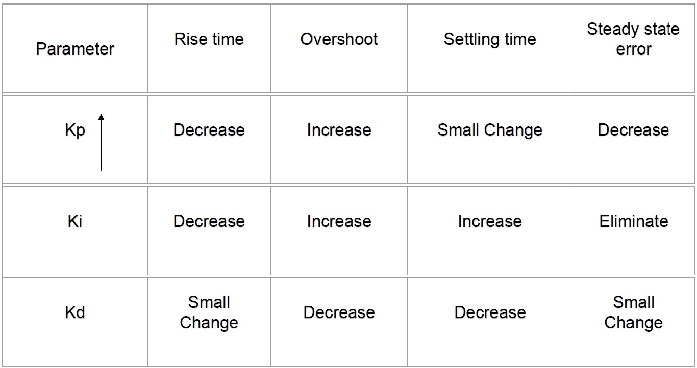
Larger $K_p$ usaully leads to faster response since the larger the error, the larger the proportional term compensation. However, an excessively large $K_p$ could cause the instability and oscillation.
The integral part is usually used for the elimination of offset caused by disturbance, etc.
The derivative part can mitigate the overshoot and stability problem arised from a proportional controller with a high gain.
The following table presents the characteristics of different part of the PID controller.
The basic routine is shown in the following table.
1. At the beginning, set all gains to zero.
2. Increase the P gain until the response to a disturbance is steady oscillation.
3. Increase the D gain until the oscillations go away (i.e. it's critically damped).
4. Repeat steps 2 and 3 until increasing the D gain does not stop the oscillations.
5. Set P and D to the last stable values.
6. Increase the I gain until it brings you to the setpoint with the number of oscillations desired (normally zero. otherwise a quicker response can be obtained if you don't mind a couple oscillations of overshoot)
Basic Knowledge of PID Control
PID control stands for the Proportional-Integral-Derivative control. We can read from its name that it consists of three parts, i.e., the proportional, integral, and derivative control. The following figure shows the structure of a system controlled by a PID controller.
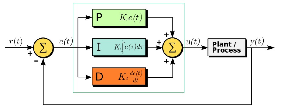
As mentioned before, the PID controller consists of three parts and it can be depicted by the following form. $$u(t)=K_pe(t)+K_i\int e(t)dt+K_d\frac{de(t)}{dt}$$ Each part has a gain parameter, denoted by $K_p$ for proportional, $K_i$ for integral, and $K_d$ for derivative, respectively. The performance of the PID controller is governed by these three gain parameters.
Larger $K_p$ usaully leads to faster response since the larger the error, the larger the proportional term compensation. However, an excessively large $K_p$ could cause the instability and oscillation.
The integral part is usually used for the elimination of offset caused by disturbance, etc.
The derivative part can mitigate the overshoot and stability problem arised from a proportional controller with a high gain.
The following table presents the characteristics of different part of the PID controller.
Parameter Tuning
One key to implement the PID controller well is the tuning of the three gain parameters. However, tuning the parameters is usually empirical and there's no formal analytical ways to do it. Many methods have been developed to faciliate the parameters tuning. Here, we present a most commonly used method.The basic routine is shown in the following table.
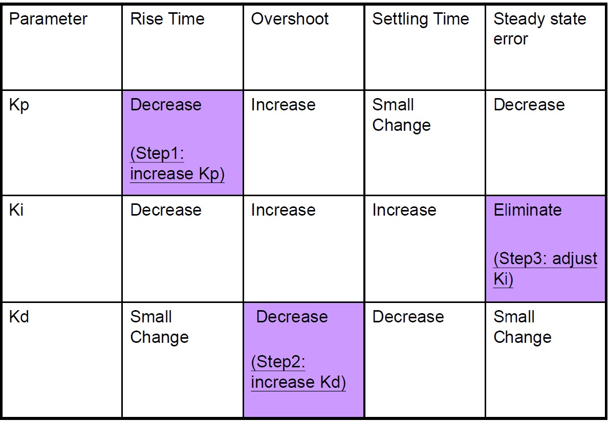
2. Increase the P gain until the response to a disturbance is steady oscillation.
3. Increase the D gain until the oscillations go away (i.e. it's critically damped).
4. Repeat steps 2 and 3 until increasing the D gain does not stop the oscillations.
5. Set P and D to the last stable values.
6. Increase the I gain until it brings you to the setpoint with the number of oscillations desired (normally zero. otherwise a quicker response can be obtained if you don't mind a couple oscillations of overshoot)
Example
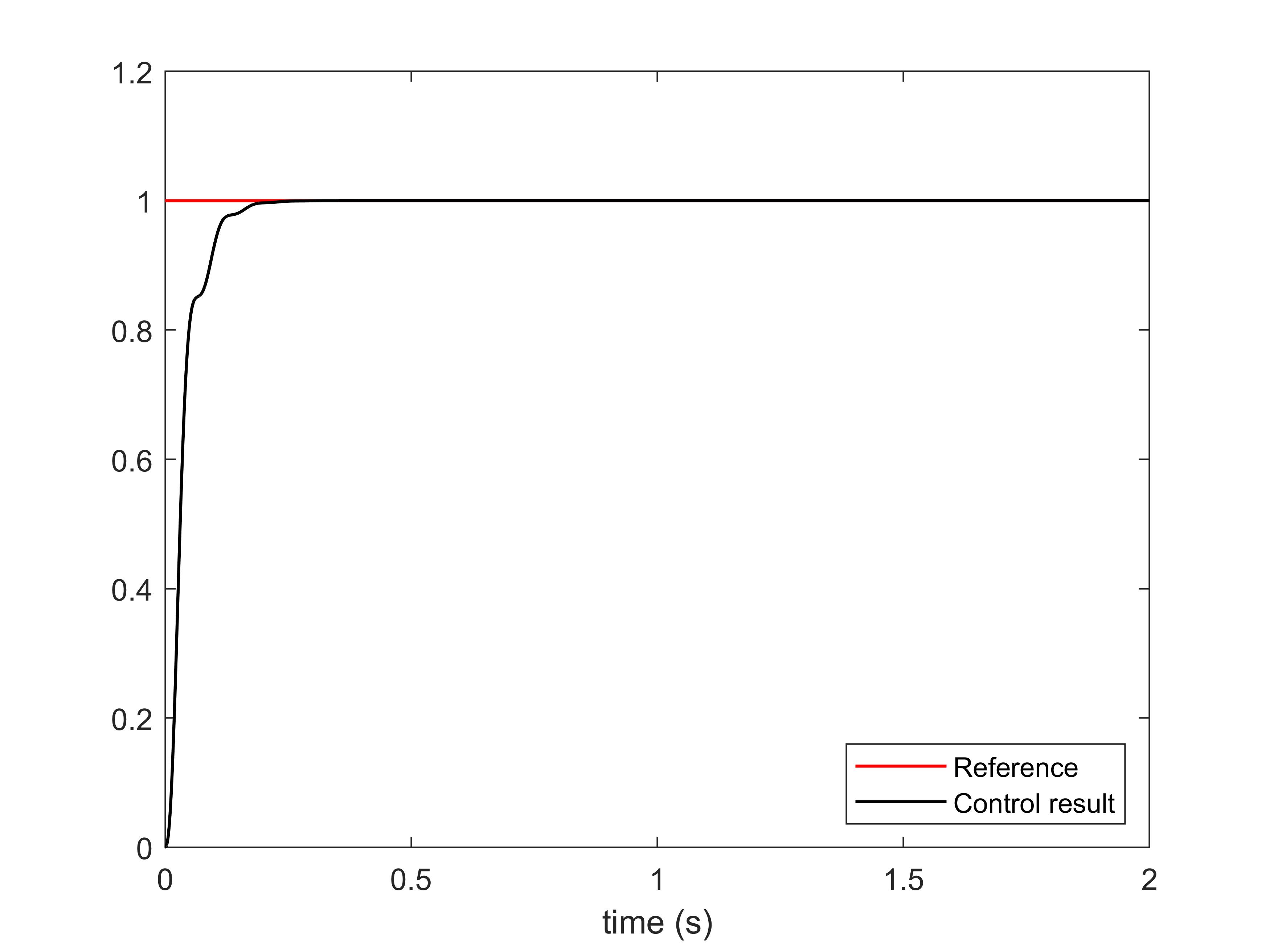
Now let us use an example to see how the implementation of PID controller works. Consider a system with the following transfer function: $$ G(s)=\frac{523500}{s^3+87.35s^2+10470s} $$ Now, we design a PID controller in the form of transfer function to drive the system to track a step signal with amplitude of 1. Create a new m file and type the following script in it, then run the script and you can obtain the simulation result.
                            close all;
                            clear;

                            % System function
                            G = tf(5.235e005,[1,87.35,1.047e004,0]);
                            % PID controller, K_p=0.5, K_i=K_d=0.001
                            G_c = tf([0.001, 0.5, 0.001], [1, 0]);

                            sys1 = series(G, G_c);
                            % Closed-loop system
                            sys2 = feedback(sys1, 1);

                            t = 0:0.001:2;
                            [y, t] = step(sys2, t);

                            plot(t, ones(size(t)), 'Color', 'r', 'LineWidth', 1)
                            hold on;
                            plot(t, y, 'Color', 'k', 'LineWidth', 1)
                            xlabel('time (s)')
                            legend('Reference', 'Control result', 'Location', 'southeast')