Advanced Matlab/Octave Tutorial -- System Analysis
Usage in Octave
To use the functions "step", "impulse", "lsim", "pole", and "pzmap" in Octave, you may need to load the control package firstly. You can add the following script to the beginning of your code to solve it.
pkg load control;
Time Responses
The time response represents how the state of a dynamic system changes in time when subjected to a particular input, such as step response, impulse response and initial condition response. For some systems, we can analytically find a closed-form solution. However, for most systems, the closed-form analytical solutions are hard to find, which brings difficulties to the analysis of their time responses. Fortunately, Matlab provides powerful tools for analyzing the time responses of dynamic systems.
Step Response
The step response of dynamic system is calculated by function "step" in Matlab. The syntax is as follows:
                                t = 0:dT:T;
                                step(sys, t);
                                t = 0:dT:T;
                                step(num, den, t);
                                t = 0:dT:T;
                                [y, t] = step(sys, t); or [y, t] = step(num, den, t);
                                plot(t, y);
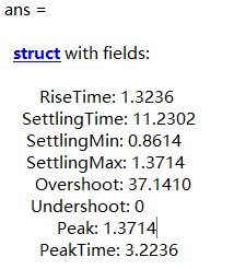
stepinfo(y, t); or stepinfo(sys);
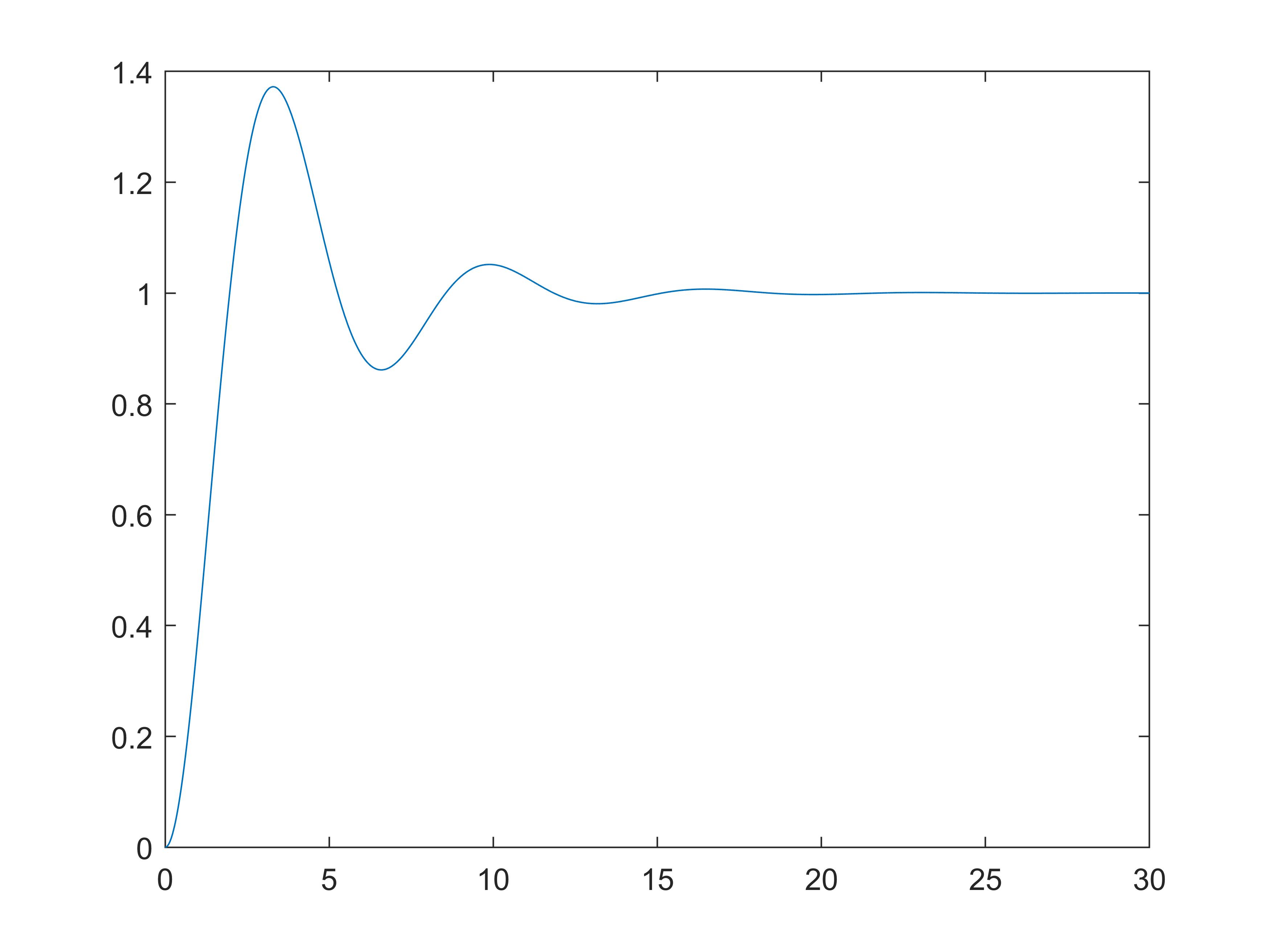
                                s = tf('s');
                                sys = 1/(s^2+0.6*s+1);

                                t = 0:0.001:30;
                                [y, t] = step(sys, t);
                                plot(t, y);
                                stepinfo(y, t)
Impulse Response
The impulse response of dynamic system is calculated by function "impulse" in Matlab. The syntax is similar to that of step response:
                                t = 0:dt:T;
                                [y, t] = impulse(sys, t); or [y, t] = impulse(num, den, t);
                                plot(t, y);
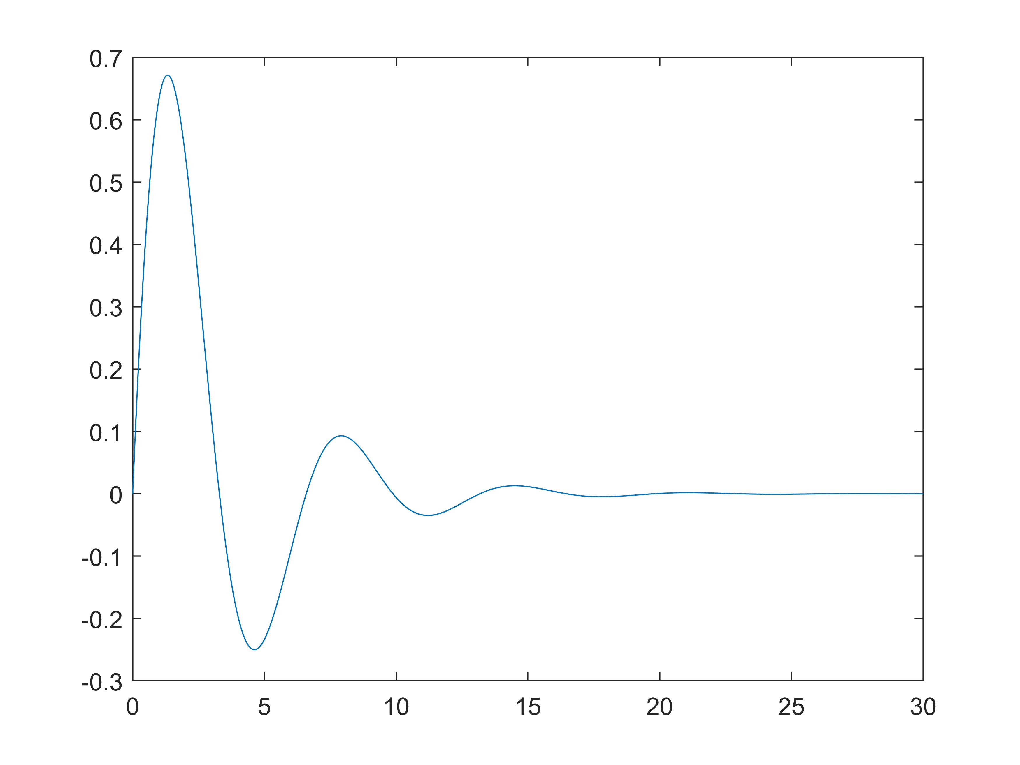
                                s = tf('s');
                                sys = 1/(s^2+0.6*s+1);

                                t = 0:0.001:30;
                                [y, t] = impulse(sys, t);
                                plot(t, y);
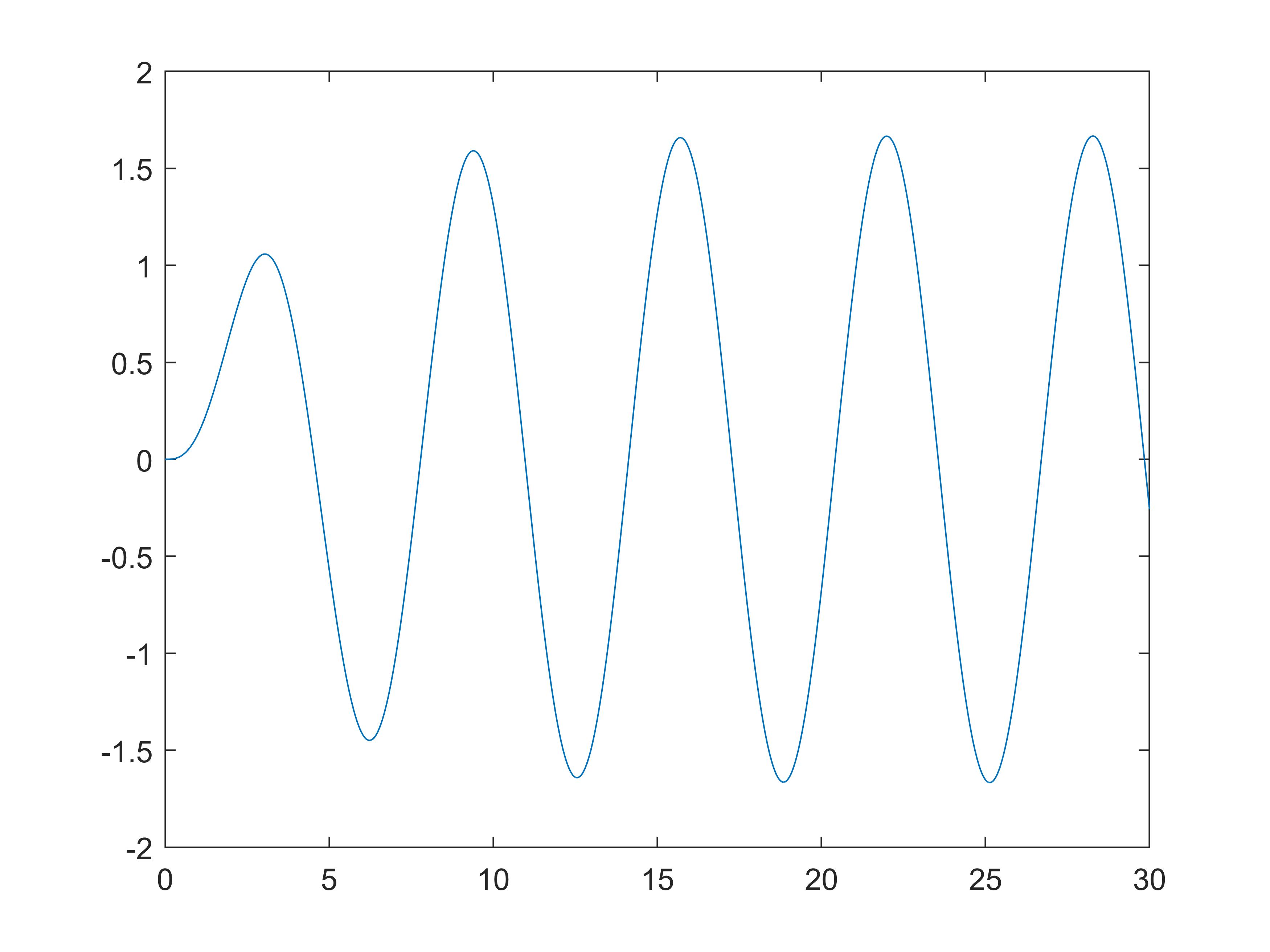
Arbitrary Input Response
The arbitrary input response of dynamic system is calculated by function "lsim" in Matlab. The syntax is as following
                                t = 0:dt:T;
                                [y, t] = lsim(sys, u, t); or [y, t] = lsim(num, den, u, t);
                                plot(t, y);
                                s = tf('s');
                                sys = 1/(s^2+0.6*s+1);

                                t = 0:0.001:30;
                                [y, t] = lsim(sys, sin(t), t);
                                plot(t, y);
Stability Analysis
As we all know, stability analysis of the dynamic systems is one of the most important problems in linear systems and control. There are many ways to analyze the stability. Matlab provides great tools for stability analysis.
Stability Analysis Based on Poles' locations
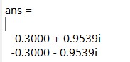
One intuitive way to analyze the stability of systems is to calculate the poles and make the analysis based on their locations. Basically, there are two methods to calculate the poles in Matlab. The first method is to use the function "roots". The syntax is as following
                                den = [denominators];
                                roots(den)
                                den = [1, 0.6, 1];
                                roots(den)
s = tf('s');
G = transFunc;
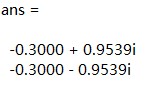
pole(G)
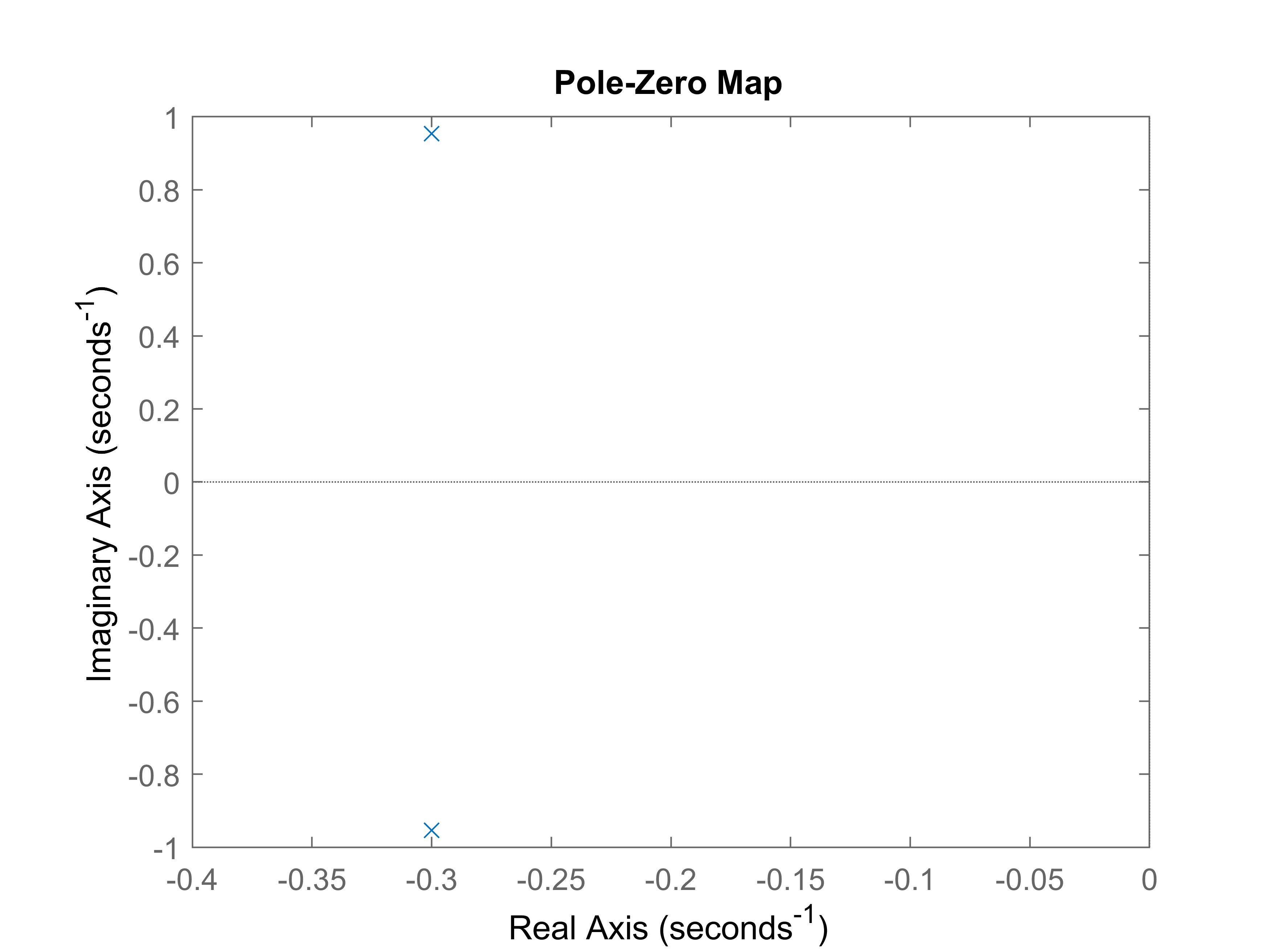
pzmap(G);
                                s = tf('s');
                                G = 1/(s^2+0.6*s+1);
                                pole(G)
                                pzmap(G);
                                axis([-0.4, 0, -1, 1]);
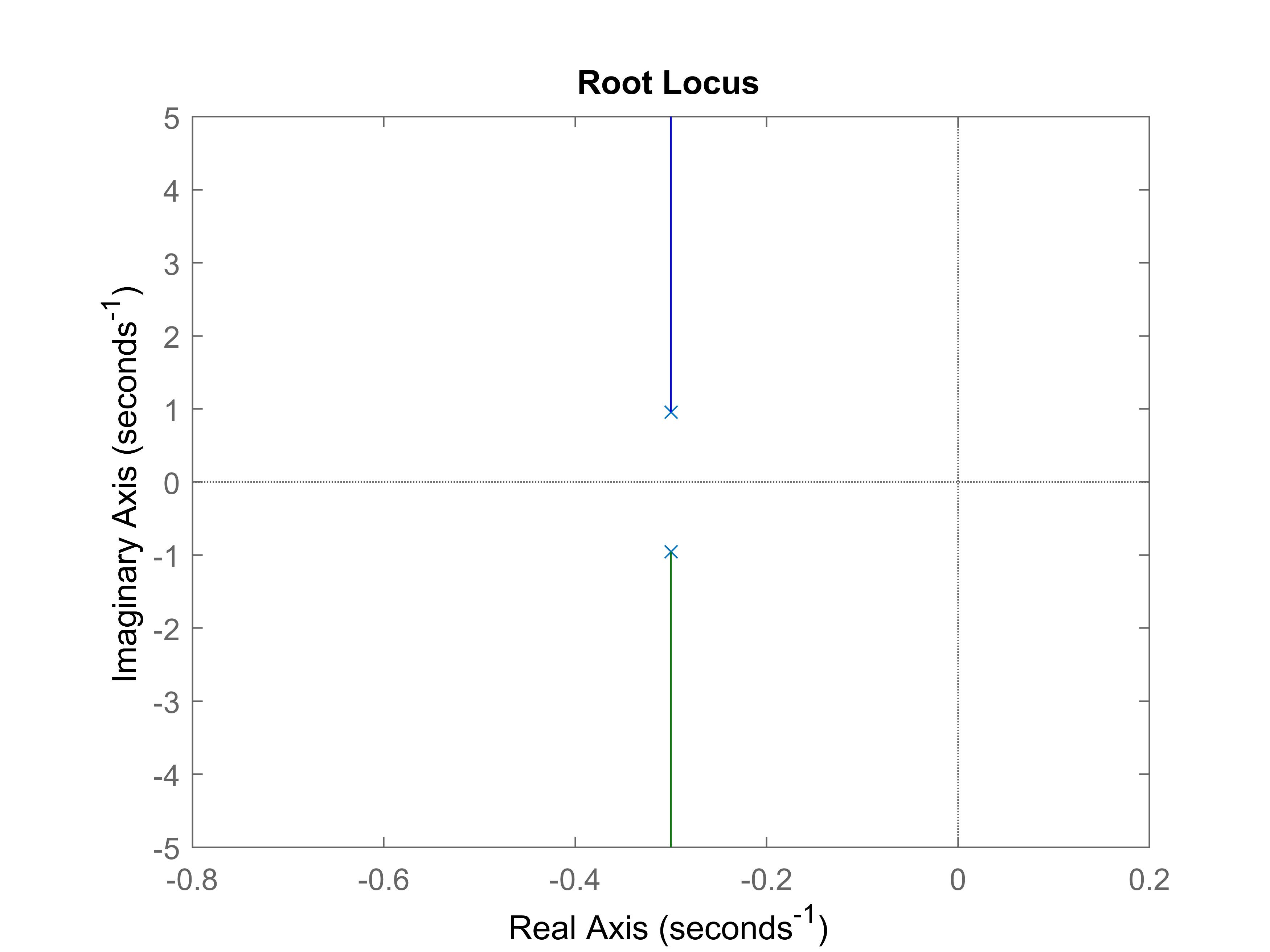
In addition, the Matlab/Octave also offer a tool to get the root locus of the system. You can achieve that by simply calling the following functon
rlocus(sys);
                                s = tf('s');
                                G = 1/(s^2+0.6*s+1);
                                rlocus(G);