Advanced Matlab/Octave Tutorial

Simulation with Transfer Functions

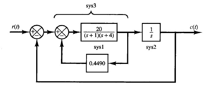
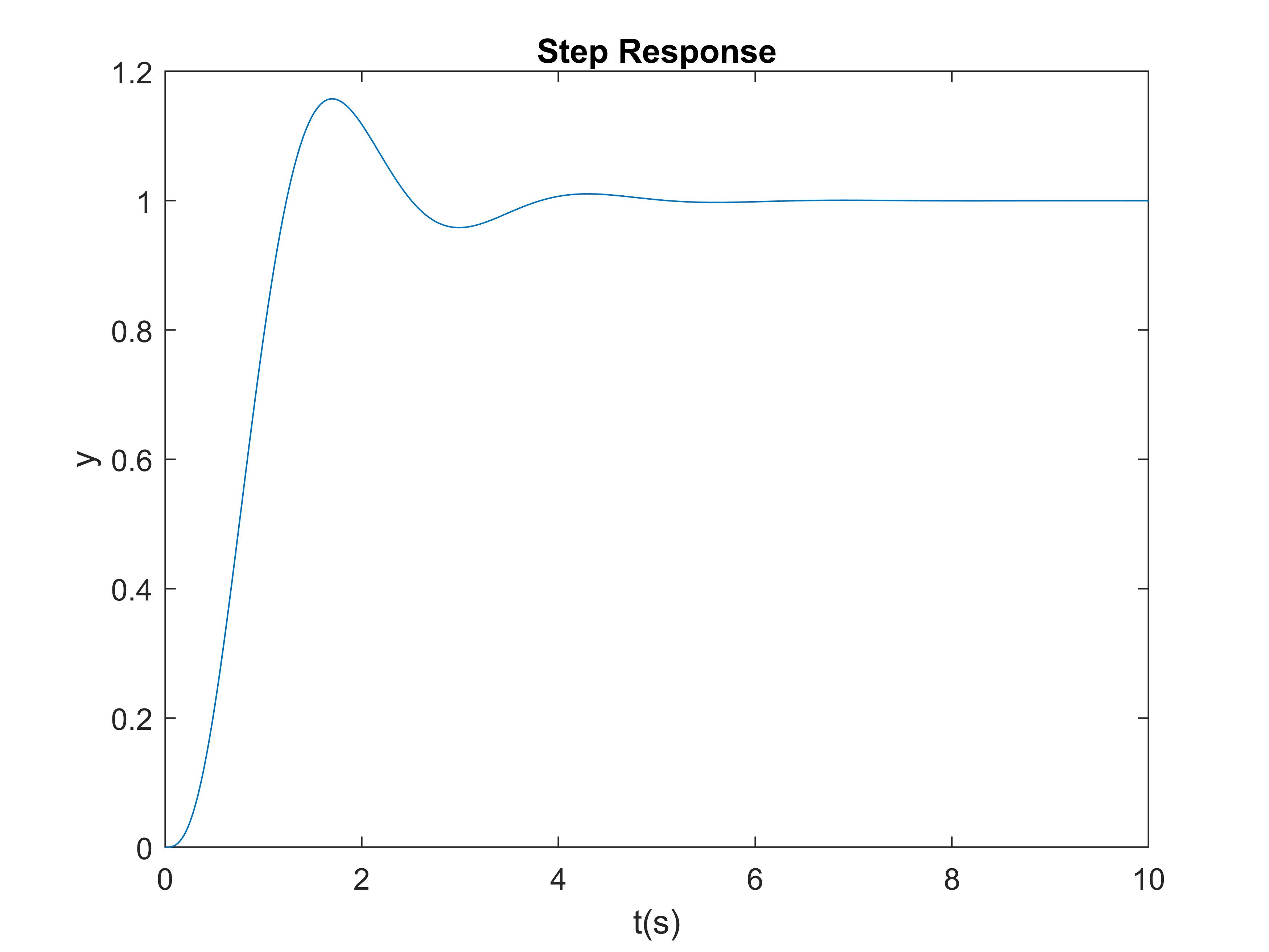
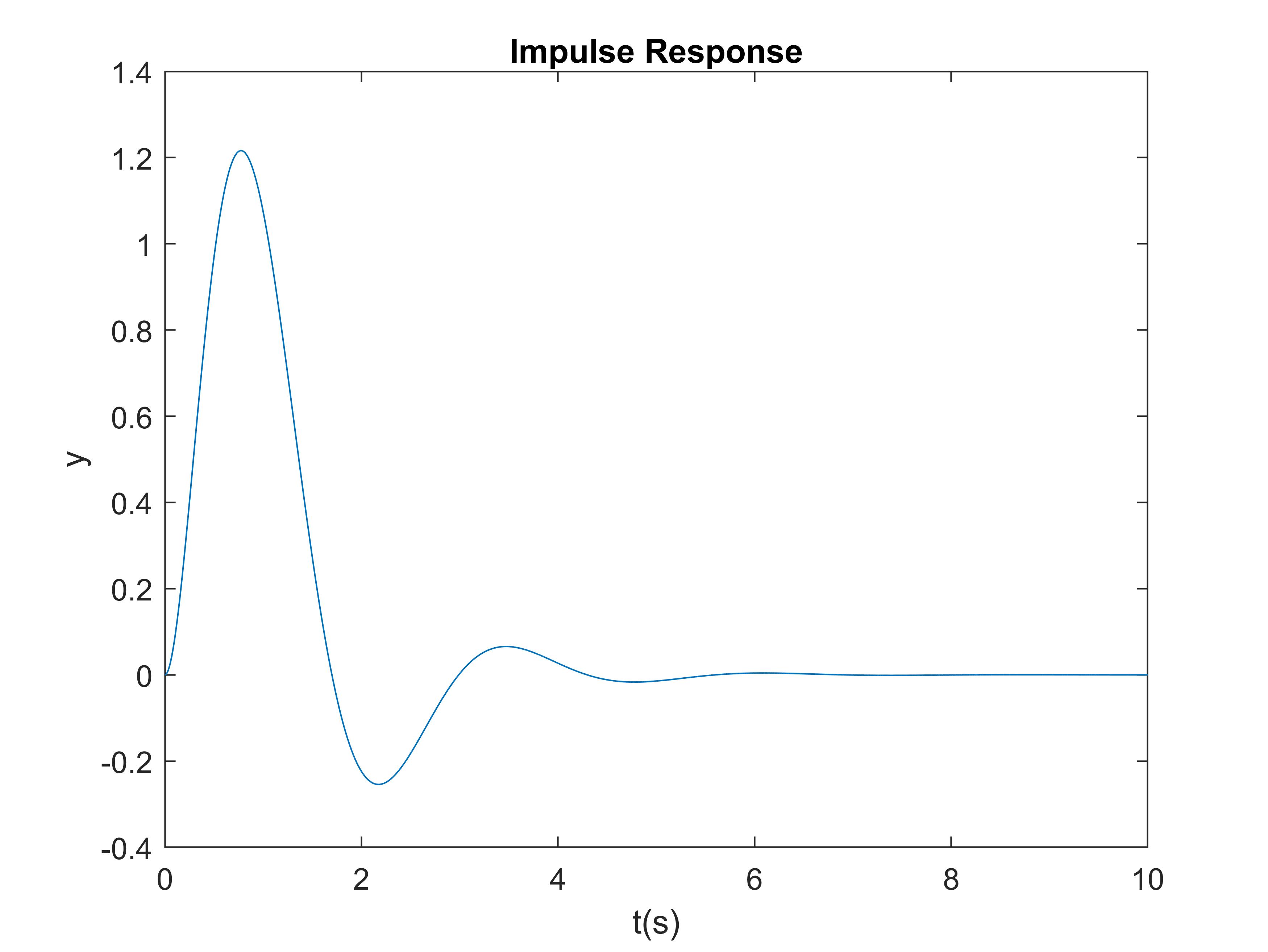
In previous sections, we have learnt how to represent a transfer function and do some simple analysis in Matlab. By now, you should be able to create simple simulations of dynamic systems as long as the transfer functions are available.

Now, let's use an example to review the previous sections. Calculate the transfer function of the following system, give the step response, impulse response and time response with a sin input, and analyze the stability of the closed-loop system.

Create a new file and type the following scripts in it.

                            clc; clear;
                            close all;

                            %% Usage in Octave
                            % Uncomment the next line to use in Octave
                            %pkg load control;

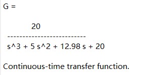
                            %% Calculate transfer function
                            s = tf('s');

                            sys1 = 20/((s+1)*(s+4));
                            h1 = 0.4490;
                            G1 = feedback(sys1, h1, -1);

                            sys2 = 1/s;
                            G2 = series(G1, sys2);

                            h2 = 1;
                            G = feedback(G2, h2, -1)

                            %% Time responses
                            t = 0:0.001:10;

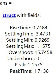
                            [y1, t] = step(G, t);
                            stepinfo(G)

                            [y2, t] = impulse(G, t);

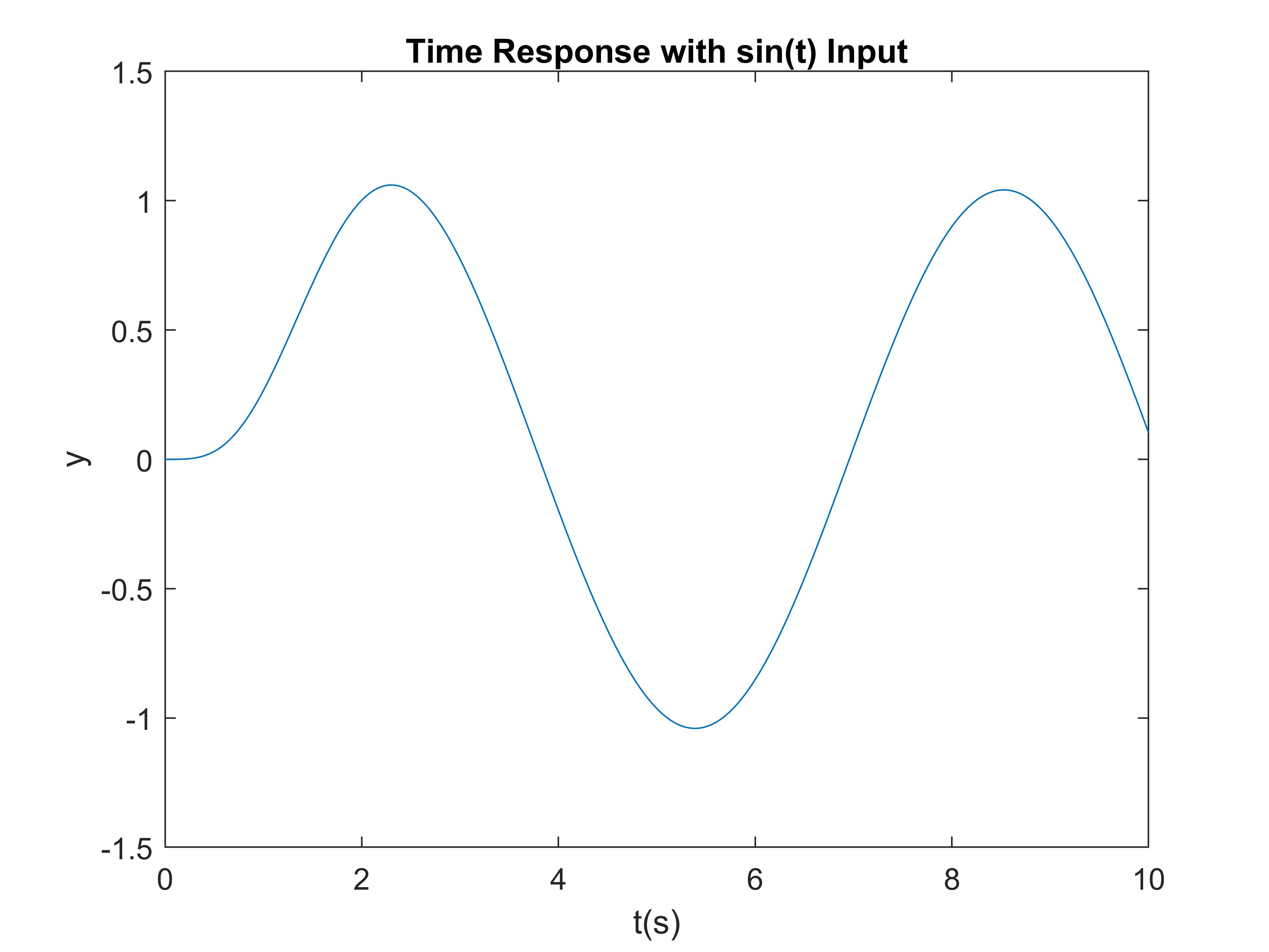
                            [y3, t] = lsim(G, sin(t), t);

                            %% Stability analysis
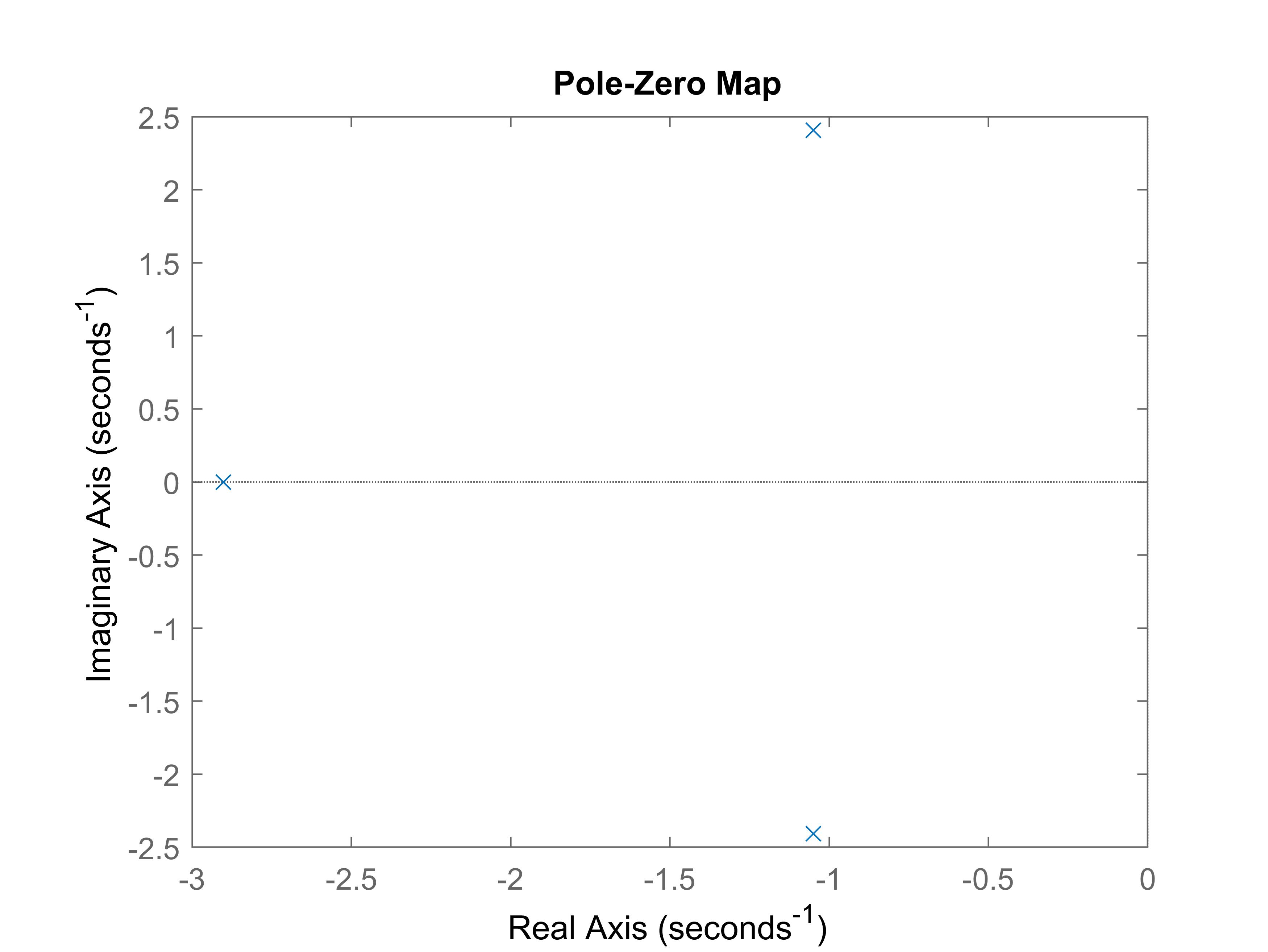
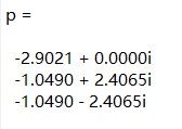
                            p = pole(G)

                            %% Plotting
                            figure(1)
                            plot(t, y1);
                            xlabel('t(s)'); ylabel('y');
                            title('Step Response');

                            figure(2)
                            plot(t, y2);
                            xlabel('t(s)'); ylabel('y');
                            title('Impulse Response');

                            figure(3)
                            plot(t, y3);
                            xlabel('t(s)'); ylabel('y');
                            title('Time Response with sin(t) Input');

                            figure(4)
                            pzmap(G);

Run the file, and you will get the results as follows:

Simulation with ODEs

Although simulation with transfer function is very convenient in Matlab, it is not enough to handle all kinds of systems. For complex systems, such as nonlinear systems, it is always the case that we can only obtain the ordinary differential equations (ODEs) but not transfer functions, and the ODEs usually cannot be analytically solved. In this case, we need to numerically calculate the ODEs instead.

Matlab provides abundant resources for numerically solving ODEs.

ODE Representation

To numerically solve the ODEs, the first step is to represent the ODEs with Matlab language. Generally, we need to create a function to represent the ODEs. The syntax is as follows.

                            function DY = Fun(t, Y)
                                ...
                                DY(1,:) = f1(Y);
                                DY(2,:) = f2(Y);
                                ...
                            end

where "t" is the time variable, "Y" is the column vector of states, and "DY" is the first derivative of "Y". For a dynamic system with control input, the syntax is as follows.

                            function DY = Fun(t, Y, u)
                                ...
                                DY(1,:) = f1(Y, u);
                                DY(2,:) = f2(Y, u);
                                ...
                            end

where "u" is the column vector of control input.

Now let's see a simple example. Create a ODE function for the following mass-damper system.

The system can be depicted by the following ODE

$$m\dot{v}+cv=f$$
Assume $m=1$ and $c=2$, the ODE can be writen as

$$\dot v=-2v+f$$
Create a new file named "dynamics.m" and type the following scripts to create the ODE function.

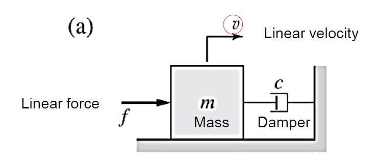
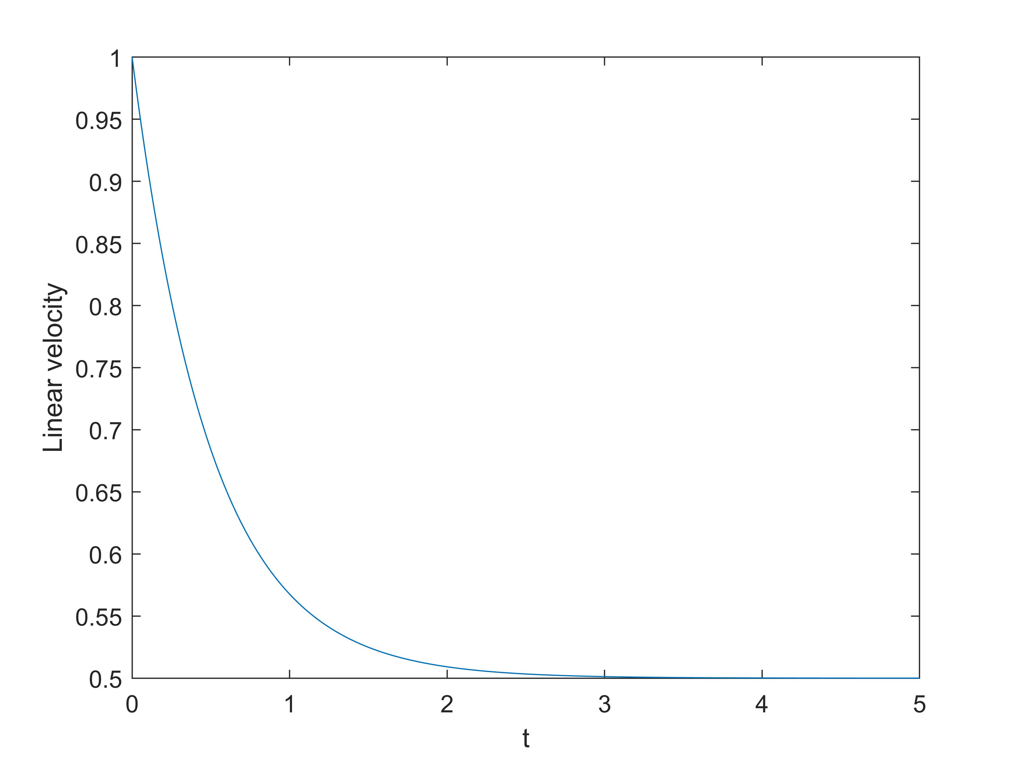
                            function dv = dynamics(t, v, f)
                                m = 1;
                                c = 2;
                                dv = -c/m*v + f;
                            end

Solvers

After we create the ODE function, we can call the solvers to solve the ODE. Matlab provides many ODE solvers. Among these solvers, the most commonly-used one is the "ode45" solver. When the ODE function is particularly expensive to evaluate, you can use "ode113" as an alternative.

The syntax of using "ode45" to solve ODE functions is

                            [t, Y] = ode45('ODE_FUN', tspan, Y0, options);

where "ODE_FUN" is the name of the ODE function file you have created, "tspan" is the time span for solving the ODE function,"Y0" is the initial value of the ODE function, "t" is the sequence of independent variable, and "Y" is the numerical solution.

"Options" is an optional argument defined by "odeset" function. The syntax of it is

                            options = odeset(Name, Value,...);

You can define many options for ODE solvers. Two commonly-used options are the error control arguments, i.e. the absolute error tolerance "AbsTol" and the relative error tolerance "RelTol".

Now, let's see an example. For the previous mass-damper system, we implement a constant force f=1 to it and create a simulation to see the time response. Create a new file and type the following scripts in it.

                            t = 0:0.001:5;
                            f = 1;
                            v0 = 1;

                            options = odeset('RelTol', 1e-6, 'AbsTol', 1e-6);
                            [~, v] = ode45(@(t, v)dynamics(t, v, f), t, v0, options);

                            figure(1)
                            plot(t, v);
                            xlabel('t'); ylabel('Linear velocity');

Note that the "@(t,v)" in the script is declaring the independent variable and state variable of the arguments of "dynamics". Run the file and you can see the figure showing the simulation result.